Profiling in Python

The last two issues mostly focused on performance of Python applications, but how do you know where your app is spending most of its time? Thats where profiling comes in. There are many approaches to profiling, here we will focus on those that are relevant to Python code and the applications we deal with day-to-day.

Put simply: if you’re interested in how long your program takes to run, you’re looking at CPU (and potentially IO) time. If you’re concerned with how much memory your program allocates during its execution, you’re looking at RAM usage.

Let’s focus on runtime for now. For the purposes of this article, we can say there two main approaches:

Deterministic Profiling

Is suitable for dev-time debugging and insights. It usually incurs some or even significant (3x slower) overhead, but provides function-level (even line-level) detail. This can be achieved by instrumenting (adding code) to the program or, in the case of Python, hooking into the interpreter itself to listen to events such as function calls, returns and exceptions.

Python has two such profilers built into the standard library, of which cProfile is the one you can use for quick access to profiling data. Simply adding python -m cProfile -o profile.prof your_program.py will create a file containing the raw data, which can be visualized using other tools we will explore next. If you need threads and asyncio support, take a look at yappi

Statistical Profiling

Is suitable even for production use and for long-running programs. It usually does not modify the running code, but instead periodically samples the program counter (“an index into the running code”) or the call stack - essentially the current line of code being executed in this instant. Over time, these snapshots build a statistical view of where the program spends most of its time.

The trade-off is that you lose insight into actual code flow, so this approach is very useful for flagging potentially problematic parts, but once you want to investigate, you will probably need to employ a deterministic profiler. Also, since these profilers effectively average out all events, they miss out on latency spikes.

Hybrid profilers

As you might expect, you can combine these two approaches and get more creative. I am including this section mainly because of scalene, which promises to do it all, even including GPU and memory - we will explore this in the future.

Visualizing the data

Once the profiler’s job is finished, we need to make sense of the data it created. Some tools have this capability built-in, most are able to export into widely compatible formats, such as callgrind and pstats. There are many tools such as snakeviz, speedscope and many others.

To give you an example, I used yappi to instrument a service I just wrote for one of our customers. I set yappi to track the “cpu” clock to ignore the network IO wait.

if __name__ == "__main__":
    yappi.set_clock_type("CPU")
    with yappi.run():
        main()
    stats = yappi.get_func_stats()
    stats.save("profile.prof", type="pstat")

I called the list_accounts capability and using gprof2dot -f pstats profile.prof > out.dot converted the pstat file into a dot file, which finally revealed the full call graph (fig 1).

When we zoom in (fig 2), we can indeed find the list_accounts function and see that the program spent 71% of the total CPU time just in that. Looking around a bit more, it seems like re.compile was called 130 times in total (fig 3), which makes out a third of our total runtime. Finally, we can take a look at the machinery of async-await (fig 4) we talked about last week, and as we might expect for such a IO bound application, there is a lot of activity in the event loop.

I hope this was a useful introduction to profiling in Python. Many of these approaches and tools also translate to other technologies, so take a look at what’s available for your tech stack.

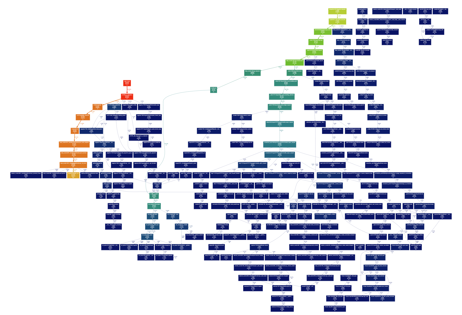fig 1. 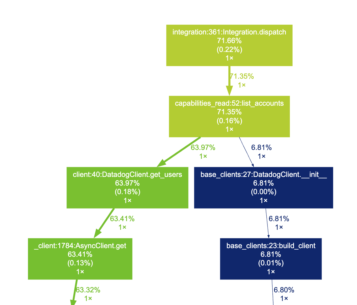fig 2. 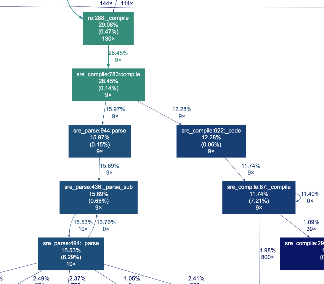fig 3. 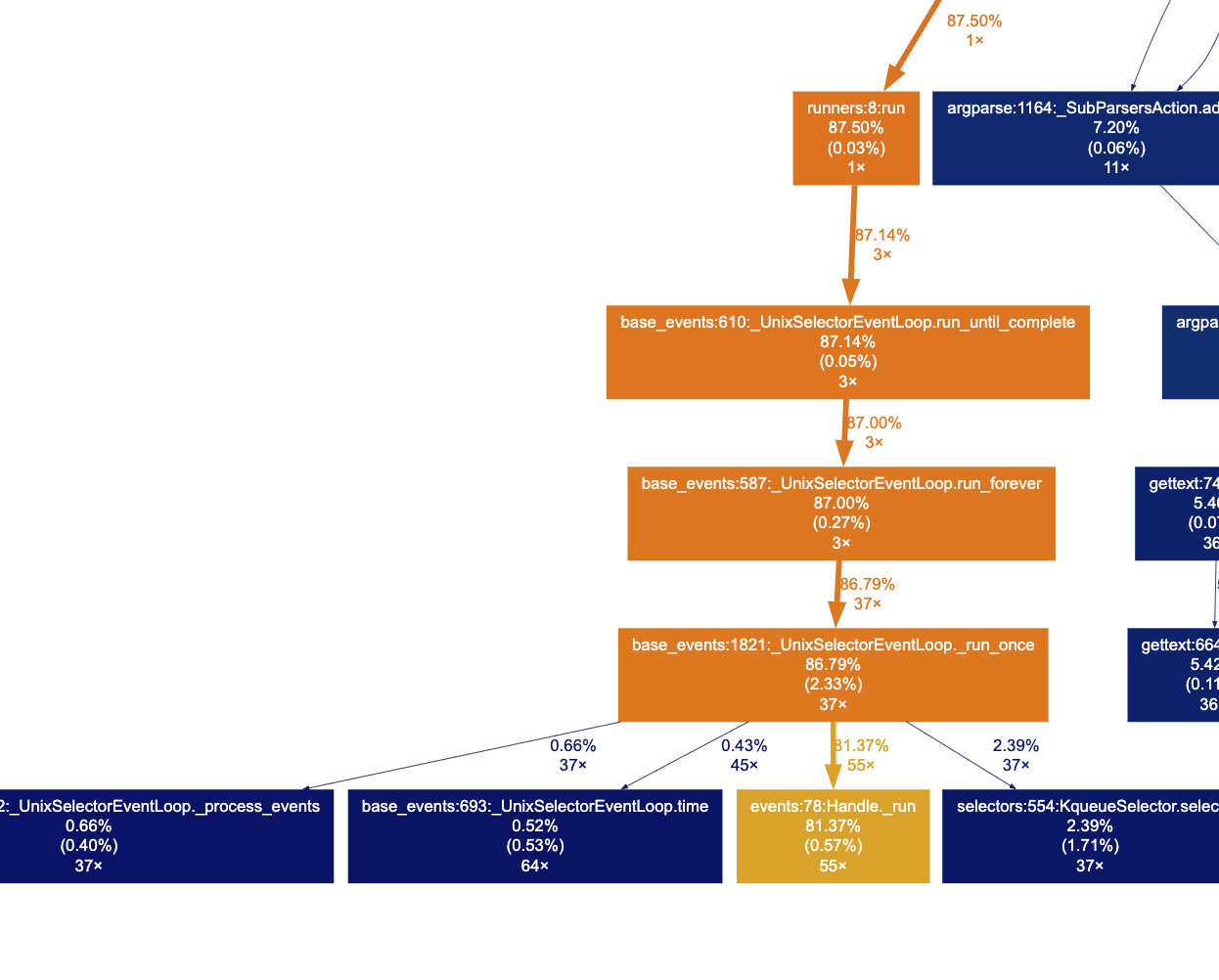fig 4.